Month: July 2025

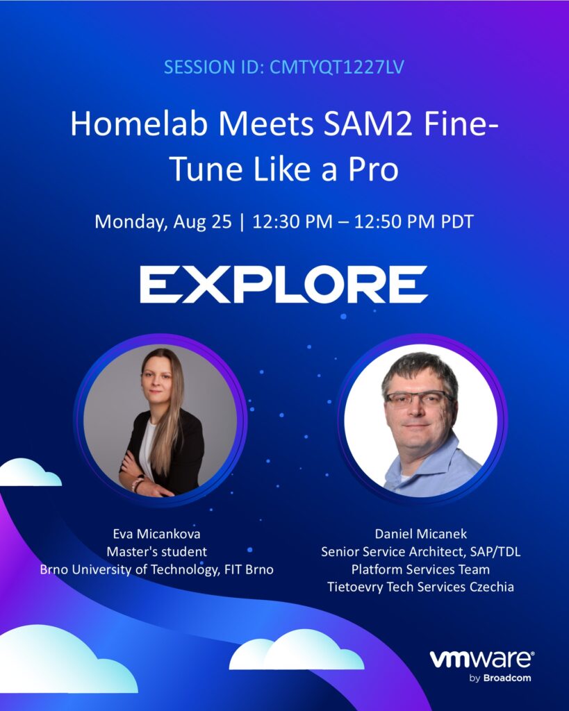
If you were at VMware Explore 2025, you might have caught our lightning talk: “Homelab Meets SAM2: Fine-Tune Like a Pro.”

In that session, I showed how the Segment Anything Model 2 (SAM2) can be adapted for interactive polyp segmentation in both images and videos. I also highlighted that SAM2 isn’t just about making your social media posts look cooler ✨ or segmenting funny-looking chickens 🐔— it also has the potential to save lives.

But like any live demo, what you saw on stage was only the tip of the iceberg. Behind the polished slides and smooth results were weeks of experimentation, GPU juggling, unexpected bugs, and plenty of “Why isn’t it learning?” moments.

This post is for those who want to dig deeper, whether you were in the room at VMware Explore or are exploring SAM2 on your own.

📝 Note: Many of the insights shared here are based on the practical experience and research from my Master’s thesis, which focused on interactive segmentation of medical video data.

SAM 2: How It’s Built

Before we dive into training details, let’s take a quick look at how Segment Anything Model 2 (SAM 2) is actually structured.

SAM 2 builds on its predecessor, Segment Anything Model (SAM), which was released by Meta AI in April 2023. While SAM was a breakthrough in interactive open-world image segmentation, it was limited to single-image inputs and lacked native support for video or sequential data. SAM 2 extends this concept by introducing architectural changes that enable it to handle both images and videos, making it suitable for tasks that require temporal consistency, such as video object segmentation and tracking.

SAM 2 is an open-source foundational model for open-world segmentation, developed and released by Meta AI in August 2024.
It was specifically designed to support interactive segmentation for both images and videos, making it one of the first models to handle temporal and spatial segmentation in a unified framework.

As an interactive model, SAM 2 accepts a wide range of user prompts — including positive and negative points, bounding boxes, and even segmentation masks. These prompts guide the model to focus on specific objects or regions, enabling precise segmentation in complex and dynamic scenes.

The Architecture That Powers SAM 2

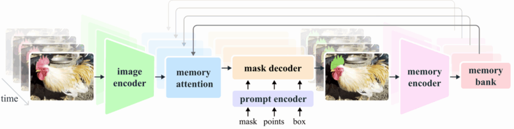
SAM 2 consists of several specialized modules that work together to enable precise and temporally consistent segmentation across both images and videos. The visualization below¹ provides a clear overview of how these components interact — from user prompts to final mask predictions, across time.

1. Source: Segment Anything Model 2 ↩︎

• Image Encoder: At its core, SAM 2 uses a transformer-based encoder to extract high-level visual features from each frame. Whether it’s a single image or a sequence of video frames, this encoder captures the spatial context and object structures at each point in time.
• Prompt Encoder: This module translates user-provided inputs – such as positive/negative clicks, bounding boxes, or coarse masks – into prompt embeddings. These embeddings guide the model to focus on specific objects or regions.
• Memory Mechanism: To enable tracking over time, SAM 2 includes a memory system composed of a memory encoder, memory bank, and attention module. This system stores relevant features from previous frames, helping the model maintain object identity even during motion, deformation, or partial occlusion.
• Mask Decoder: The decoder fuses all information – visual features, prompt embeddings, and memory context – to produce the final segmentation mask. In video mode, it leverages stored memory to ensure that objects are segmented consistently across frames

From General to Specific: Fine-Tuning SAM 2

While SAM 2 is trained on the massive and diverse SA-V dataset, making it a powerful generalist, real-world applications often require greater precision and consistency. When the model is applied to a domain that was not well-represented in the original training data — such as medical imaging or other highly specialized fields — its out-of-the-box performance may fall short.

That’s where fine-tuning comes in.

The Meta AI team provides official training and fine-tuning code for SAM 2, including detailed instructions in the training README. However, based on my experience, this codebase is quite complex and optimized for large-scale multi-GPU setups. Since I was working with a domain-specific dataset and didn’t require distributed training, I needed more granular control over the training loop and fine-tuning process. That’s why I chose to write my own simplified fine-tuning pipeline — tailored to single-GPU setups and easier to adapt to custom datasets. I’m sharing this approach here in the hope that it will be helpful for others facing similar challenges.

Fine-Tuning SAM 2 for Interactive Image Segmentation with Bounding Box Prompts

Before we begin fine-tuning, several preparation steps are required.
First, we need to load the pretrained SAM 2 model. After that, we selectively enable the components we wish to fine-tune (e.g., image encoder, prompt encoder, or mask decoder). Next, we choose an appropriate loss function and optimizer based on our task and dataset. Once all components are in place, we can implement the training loop, including the forward pass and backpropagation.

For a practical introduction to how SAM 2 can be used on static images, the official SAM2 GitHub repository provides ready-to-run Jupyter notebooks. A good starting point is the image_predictor_example.ipynb, which demonstrates how to load the model, apply prompts, and generate segmentation masks.

1. Loading the Pretrained SAM 2 Model

To use Segment Anything Model 2 (SAM 2), we first need to build the model architecture and load its pretrained weights. This is done using the build_sam2 function and the SAM2ImagePredictor wrapper:

from sam2.build_sam import build_sam2
from sam2.sam2_image_predictor import SAM2ImagePredictor

sam2_checkpoint = "../checkpoints/sam2.1_hiera_small.pt"
model_cfg = "configs/sam2.1/sam2.1_hiera_s.yaml"

predictor = build_sam2(model_cfg, sam2_checkpoint, device=device)

• model_cfg: Path to the YAML configuration file describing the architecture of the desired SAM 2 variant
• sam2_checkpoint: Path to the corresponding pretrained model weights (.pt checkpoint).
• build_sam2(...): Constructs the SAM 2 model and loads its weights.
• SAM2ImagePredictor(...): Wraps the model in a high-level inference class that simplifies interaction.

2. Enabling Model Components for Fine-Tuning

When fine-tuning SAM 2 for image segmentation, the three essential components that can be trained are:

• predictor.model.image_encoder
• predictor.model.sam_prompt_encoder
• predictor.model.sam_mask_decoder

Each of these modules can be selectively enabled for training based on your configuration and GPU capacity.

These components are implemented in PyTorch and can be selectively enabled for training. To fine-tune any of them, you need to set the module to training mode using .train(True) and ensure all parameters have requires_grad = True. For example:

predictor.model.sam_mask_decoder.train(True)
for p in predictor.model.sam_mask_decoder.parameters():
    p.requires_grad = True

⚠️ Note: Be sure to comment out any @torch.no_grad() or @torch.inference_mode() decorators in the source code — particularly in the ./sam2 folder (sam2_image_predictor.py) of the repository. These decorators are designed to speed up inference by disabling gradient tracking and certain computation paths, but they will prevent training from working correctly.

3. Defining the Loss Function

To compute the difference between predicted masks and ground-truth masks, we need a suitable loss function. A convenient option is to use the segmentation_models_pytorch (SMP) library, which provides ready-to-use implementations of popular segmentation loss functions such as DiceLoss, FocalLoss, or combinations thereof.

In my own experiments, I used Dice Loss, as it is well-suited for segmentation tasks with imbalanced foreground and background pixels—a common scenario in medical imaging. However, depending on your dataset and goals, you may want to experiment with other loss functions like Binary Cross-Entropy, Focal Loss, or custom hybrids.

4. Selecting the Optimizer

Once the model and loss function are defined, the next step is to select an optimizer that will update the model’s parameters during training. In most PyTorch-based workflows, popular choices include SGD, Adam, and AdamW.

For my experiments, I used AdamW, which is a variant of the Adam optimizer with decoupled weight decay. It often works well in computer vision tasks and provides better generalization, especially when fine-tuning large pretrained models like SAM 2.

In my fine-tuning setup, I assigned different learning rates and weight decay values to individual components of the SAM 2 model. Specifically, I used a lower learning rate (1e-6) for the image encoder, since it is a large and sensitive component pretrained on diverse data. For the prompt encoder and the mask decoder, I used a slightly higher learning rate (5e-6), which allowed them to adapt more quickly to the target task. For all components, I applied a weight decay of 1e-4 to encourage regularization and improve generalization. This configuration proved effective in practice and led to stable training across multiple datasets.

5. Implementing the Training Loop

Once all components are prepared—model, optimizer, and loss function—we can implement the training loop:

preds = sam2_forward_pass(...)

preds = preds.to(dtype=torch.float32)
masks = masks.to(dtype=torch.float32)

loss_value = loss(preds, masks)

optimizer.zero_grad()
loss_value.backward()
optimizer.step()

During each iteration we first perform a forward pass using sam2_forward_pass(...) to obtain predicted masks. Both the predictions and ground-truth masks are then cast to float32, ensuring they are compatible for loss computation.

The loss is computed using the selected loss function (e.g., DiceLoss), and we then proceed with the standard PyTorch optimization routine: we reset gradients with optimizer.zero_grad(), perform backpropagation via loss_value.backward(), and update the model parameters using optimizer.step().

This training step is typically wrapped inside an epoch loop and may be extended with gradient accumulation, learning rate scheduling, or mixed-precision training as needed.

6. Writing the SAM 2 Forward Pass

Now lets dive into the forward pass implementation.

⚠️ Note: Be sure to comment out any @torch.no_grad() or @torch.inference_mode() decorators in the source code — particularly in the ./sam2 folder (sam2_image_predictor.py) of the repository. These decorators are designed to speed up inference by disabling gradient tracking and certain computation paths, but they will prevent training from working correctly.

First, we pass the input image batch through the SAM 2 image encoder. This step extracts high-level visual features from each image, which will later be combined with prompt embeddings to guide the segmentation process.

predictor.set_image_batch(images_list)

The images_list is expected to be a list of NumPy arrays, where each image has shape [H, W, C] (Height, Width, Channels) and is typically of type float32.
The list itself emulates the batch dimension, allowing multiple images to be processed together.

Next, we prepare the prompt input — in this case, bounding boxes:

_, _, _, unnorm_box = predictor._prep_prompts(
                 point_coords=None, 
                 point_labels=None, 
                 box=bbox_coords,
                 mask_logits=None, 
                 normalize_coords=True
                 )

The variable bbox_coords contains the box coordinates in unnormalized format [x1, y1, x2, y2], where the values are in pixel units relative to the original input image size. These coordinates will be normalized internally by the model before being passed to the prompt encoder.

The prepared box coordinates are passed into the prompt encoder to obtain both sparse and dense embeddings:

sparse_embeddings, dense_embeddings = predictor.model.sam_prompt_encoder(
                 points=None, 
                 boxes=unnorm_box, 
                 masks=Non
                 )

We also extract high-resolution image features, which are used to improve the accuracy of mask decoding:

high_res_features = [feat_level[-1].unsqueeze(0) for feat_level in predictor._features["high_res_feats"]]

The mask decoder combines all inputs to predict segmentation masks:

low_res_masks, _, _, _ = predictor.model.sam_mask_decoder(
                image_embeddings=predictor._features["image_embed"],
                image_pe=predictor.model.sam_prompt_encoder.get_dense_pe(),
                sparse_prompt_embeddings=sparse_embeddings,
                dense_prompt_embeddings=dense_embeddings,
                multimask_output=True,
                repeat_image=False,
                high_res_features=high_res_features,
                )

Finally, the predicted masks are upsampled to the desired resolution (e.g. 512×512) and passed through a sigmoid activation to obtain per-pixel probabilities:

preds = predictor._transforms.postprocess_masks(low_res_masks, img_size) # output image size (e.g. 512)
preds = torch.sigmoid(preds[:, 0])

Since the model is configured with multimask_output=True, the mask decoder produces three candidate masks for each image. For fine-tuning, we only use the first output mask (index 0), which is usually the most relevant. This is done by slicing with preds[:, 0], reducing the shape from [B, N, H, W] to [B, H, W], where N is the number of masks per image. Applying torch.sigmoid then converts the raw logits into probability values.

Domain-Specific Video Segmentation with SAM 2 and Box Prompts

Alright, now that we’ve covered the essential components of fine-tuning SAM 2 for static images, let’s dive into video segmentation. Fortunately, many of the building blocks from the previous chapter — such as the loss function and optimizer — remain applicable. In this section, we’ll explore how to adapt the fine-tuning pipeline to work with video data using bounding box prompts.

For a practical introduction to how SAM 2 can be applied to video data, the official SAM 2 GitHub repository also includes a ready-to-run notebook for video segmentation. The video_predictor_example.ipynb demonstrates how to process a sequence of frames, apply prompts, and generate segmentation masks consistently across time. It’s a great starting point for understanding how SAM 2 handles video inputs and temporal context.

Similarly to the image-based setup, we need to go through several key steps: loading the same pretrained checkpoint used by the video predictor, enabling the desired model components for training, and defining a forward pass tailored for video inputs. Each of these steps builds upon the foundations we covered earlier, but with adjustments to handle sequential data and temporal dynamics.

⚠️ Note: In my own experiments, I fine-tuned SAM 2 for video segmentation using a custom approach tailored to my specific dataset. The recommendations in this section are based on what worked best for me in practice. I was working with sparsely annotated video sequences, where only a few frames had ground-truth masks available. To address this, I created training sequences of variable length — typically between 1 and 4 frames — and computed the loss only on the final frame of each sequence. This setup allowed the model to learn prompt propagation over time, while making the most out of limited annotations. In my experience, this approach led to more stable training and better generalization than using fixed-length sequences or computing loss on all frames.

1. Loading the Pretrained SAM 2 Checkpoint for Video

To begin fine-tuning SAM 2 for video segmentation, we first load the pretrained model in video mode using the build_sam2_video_predictor function. This function initializes the model with support for sequential frame processing and enables video-specific features such as temporal embeddings.

from sam2.build_sam import build_sam2_video_predictor

sam2_checkpoint = "../checkpoints/sam2.1_hiera_small.pt"
model_cfg = "configs/sam2.1/sam2.1_hiera_s.yaml"

predictor = build_sam2_video_predictor(model_cfg, sam2_checkpoint, device=device)

2. Trainable Modules in SAM 2 for Video Segmentation

When fine-tuning SAM 2 for video segmentation, the model includes several additional components specifically designed to handle temporal information. The following modules can be selectively enabled for training:

• predictor.image_encoder – extracts visual features from each frame (same as in the image version),
• predictor.sam_prompt_encoder – encodes prompts such as boxes or points,
• predictor.sam_mask_decoder –generates segmentation masks from combined image features, prompt embeddings, and temporal memory,
• predictor.memory_encoder – encodes past frame information to provide temporal context,
• predictor.memory_attention – applies attention over temporal memory to support consistent object tracking,
• predictor.obj_ptr_proj – projects memory features for object pointer modeling,
• predictor.obj_ptr_tpos_proj – encodes temporal positional embeddings for object-level temporal reasoning.

These components work together to enable temporally consistent predictions across video frames. Since the model is based on PyTorch, fine-tuning any of these parts requires setting them to training mode using .train(True) and ensuring their parameters have requires_grad = True. This allows gradients to flow and weights to update during backpropagation:

predictor.memory_encoder.train(True)
for p in predictor.memory_encoder.parameters():
    p.requires_grad = True

⚠️ Note: Be sure to comment out any @torch.no_grad() or @torch.inference_mode() decorators in the source code — particularly in the ./sam2 folder (sam2_video_predictor.py) of the repository. These decorators are designed to speed up inference by disabling gradient tracking and certain computation paths, but they will prevent training from working correctly.

3. Forward Pass for Video Segmentation with SAM 2

The video forward pass in SAM 2 requires more preparation than static image inference, as it handles multiple frames, memory management, and prompt propagation across time. The process is encapsulated in two functions: create_inference_state(...) and sam2_forward_pass(...).

Understanding and Customizing init_state()

Before implementing the forward pass, I highly recommend taking time to understand how the SAM2VideoPredictor works internally — especially the init_state() function. This method is responsible for creating the inference state, a central structure that stores everything SAM 2 needs to track and segment objects across video frames.

For training purposes, you’ll likely need to adapt this logic — especially to:

• load frames and annotations from tensors or memory instead of a video path,
• work with variable-length sequences, not full videos,
• and adjust the input resolution (image_size) to match your training pipeline.

In my case, I implemented a simplified version of init_state() that accepts a preloaded batch of frames (from sequence_data) and integrates seamlessly with my training loop. This gave me full control over how sequences are formed, annotated, and processed during fine-tuning.

⚠️ Code Modification
In order to get fine-tuning working correctly, I also had to modify line 794 in SAM2VideoPredictor.
Originally, the code assumes that object_score_logits is always present:

object_score_logits = current_out["object_score_logits"]

However, during training with custom data or partial inputs, this key may be missing. To prevent errors and ensure the forward pass still works, I replaced it with a safe fallback:

object_score_logits = current_out.get("object_score_logits", torch.ones(1, 64, device=current_out["pred_masks"].device))

This creates a dummy tensor when the score logits are not available, allowing the training process to proceed without crashing.

Putting It All Together: The Forward Pass for Video

Before running the forward pass, we first initialize a fresh inference state using our custom create_inference_state(...) function — a reimplementation of SAM 2’s original init_state(), adapted for training. This prepares all necessary structures for tracking, memory, and prompt inputs.

inference_state = create_inference_state(...)
predictor.reset_state(inference_state)

After creating the state, we call predictor.reset_state(...) to ensure the model starts with a clean internal memory. This is important to avoid any residual data from previous sequences during training or evaluation.

With the inference state initialized and reset, we can now run the forward pass for the current video sequence. We start by injecting the initial prompt — in this case, a bounding box — into the first frame (ann_frame_idx = 0) using predictor.add_new_points_or_box(...). This establishes the object we want to segment and track throughout the video.

ann_frame_idx = 0
ann_obj_id = 1
    
_, out_obj_ids, out_mask_logits = predictor.add_new_points_or_box(
            inference_state=inference_state,
            frame_idx=ann_frame_idx,
            obj_id=ann_obj_id,
            box=sequence_data["prompt_bbox"]
)
    
video_segments = {}  # Video_segments contains the per-frame segmentation results

If the sequence contains multiple frames, the model then propagates the object across the video using memory attention via predictor.propagate_in_video(...). This produces a set of predicted masks for each frame.

Finally, all masks are stacked and passed through a sigmoid to obtain per-pixel probabilities. The output preds has the shape [T, C, H, W], where T is the number of frames.

if inference_state["num_frames"] > 1:
    for out_frame_idx, out_obj_ids, out_mask_logits in predictor.propagate_in_video(inference_state):
        video_segments[out_frame_idx] = {
            out_obj_id: out_mask_logits[i]
            for i, out_obj_id in enumerate(out_obj_ids)
        }
        
    # Return video segments in shape: [T,C,H,W]
    preds = torch.stack([torch.sigmoid(segment[ann_obj_id]) for segment in video_segments.values()]).to(device)
else:
    # Return video segments in shape: [T,C,H,W]
    preds = torch.sigmoid(out_mask_logits).to(device)

Final Notes

While implementing the forward pass, you may have noticed a potential limitation — all frames in the sequence are loaded into memory at once. This is not ideal for longer videos or real-time applications. Fortunately, there is an alternative implementation of SAM 2 designed for streaming input: segment-anything-2-real-time.

This real-time version of SAM 2 is optimized for sequential frame-by-frame processing and significantly reduces memory usage. The fine-tuned model you trained following this guide can be integrated into that pipeline, making it suitable for deployment in low-latency or resource-constrained environments.

I hope this walkthrough helped clarify how SAM2 can be fine-tuned for both image and video segmentation — and that it gave you a clearer path for applying it to your own project or research. If you have any questions, run into unexpected issues, or just want to share what you’re working on, feel free to reach out. I’ll be happy to help or discuss further. If you’re interested in a deeper dive into the methods and experiments behind this work — particularly in the context of medical video segmentation — feel free to check out my Master’s thesis, where many of these insights originated.

Good luck, and happy segmenting!